Focal loss gamma for a small language model: the math, the code, and how I use it
Short version: I train my small language models with focal loss instead of plain cross-entropy. Focal loss is one extra multiplier on each token's loss, (1 - p)^γ, that shrinks the contribution of tokens the model already predicts with confidence. The idea is not mine. It comes from the RetinaNet paper, "Focal Loss for Dense Object Detection" (Lin, Goyal, Girshick, He and Dollár, 2017), where it was built for object detection. This post puts cross-entropy and focal loss side by side, in math and in PyTorch, shows the three things I added to make it work for language model training, and ends with how I would suggest setting gamma. This is a personal project built on personal time with personal resources.
A note on how I work, since this post has formulas in it: I am a builder, not a mathematician. I work from code and experiments. The formulas are here for readers who want them, and each one is backed by code in this post that you can run.
Where this code lives
Everything here is part of make_your_own_llm, my project for building small language models from scratch: the data pipeline, the tokenizer, the model and the training loop. That repository is private, so there is nothing to clone. The code in this post is copied out of it.
Focal loss has been in that project since March 5, 2026, the day of the commit titled "implement focal loss gamma", and it has been part of my training setup ever since. Both released Peacebell models were trained with it:
- Peacebell v1 291M: https://huggingface.co/wayneworkman2012/peacebell-v1-291M
- Peacebell v1 148M: https://huggingface.co/wayneworkman2012/peacebell-v1-148M
The two models I am working on now use the same approach. I expect to release them on my Hugging Face account in the coming weeks, at these addresses (not live yet):
wayneworkman2012/boris2-peacebell-base: https://huggingface.co/wayneworkman2012/boris2-peacebell-basewayneworkman2012/boris2-peacebell-instruct: https://huggingface.co/wayneworkman2012/boris2-peacebell-instruct
They are a Peacebell-architecture version of Boris-2. Thank you to Joseph Jones, the creator of Boris, for letting me make it. The original Boris-2 instruct model is here: https://huggingface.co/opencerebral/Boris-2-Instruct
Credit where it is due
Focal loss was introduced by Tsung-Yi Lin, Priya Goyal, Ross Girshick, Kaiming He and Piotr Dollár in "Focal Loss for Dense Object Detection" (ICCV 2017), the paper that also introduced the RetinaNet detector. Their problem was class imbalance in object detection. A detector scores a huge number of candidate locations per image, almost all of them are easy background, and the sheer count of easy examples swamps the loss. Their fix was to multiply cross-entropy by (1 - p)^γ so that well-classified examples count for less. They report that γ = 2 worked best in their experiments, and their own example is the cleanest summary of the effect: with γ = 2, an example classified at p = 0.9 has about 100 times lower loss than it has under cross-entropy.
To be plain about what belongs to whom in this post:
From the paper, not mine:
- The focal loss formula and its modulator,
(1 - p)^γ. - The whole idea of downweighting examples the model already gets right.
- 2.0 as the value of gamma. It is the value they report worked best.
- The gradient of the focal loss. Their Appendix B gives it for their binary case, and the form in this post is the same expression written for a softmax.
- Using it across many classes. Their loss is written for binary classification on sigmoid outputs, and a footnote in the paper says that extending it to the multi-class case is straightforward. A softmax over a vocabulary, with
pas the probability of the correct next token, is that extension. - The loss chart further down. I drew it from their formula, and it is the same kind of plot as their Figure 1.
Standard material, not mine and not theirs:
- Cross-entropy, softmax and the cross-entropy gradient.
- Clamping a value away from zero to keep a gradient finite. That is a routine numerical guard.
Mine:
- The implementation in my project, which is the code shown here.
- Changing gamma during a run from my training schedule, and the shape of that schedule. I make no claim that varying gamma during training is new. Other people have published ways of doing it, for example AdaFocal (Ghosh, Schaaf and Gormley, NeurIPS 2022). Mine is what I built for my own runs.
- Finding out the hard way that gamma below 1 needs that guard.
- Taking the logged cross-entropy from the focal pass itself.
- The comparison against gamma 0, and the opinions at the end.
I also make no claim to be the first to use focal loss on text, and I do not use the paper's class-balancing weight, alpha.
None of this is a new loss. It is their loss, used for next-token prediction.
Why I wanted it
My commit log from that week shows what I was looking at. On February 28 I wrote a per-token loss analysis script, to see which tokens the model struggled with most. On March 1 I counted how often each token of my vocabulary appears in the training data, and started generating extra training examples for the rare ones. One of the first I worked on was the word "speakeasies", which the corpus barely contained. That attacks rare tokens from the data side. Focal loss attacks the same thing from the loss side, and it went in four days later.
The worry is simple to state. A language model sees a great many tokens that become easy early: punctuation, function words, the second half of a word once the first half is on the page. On a domain corpus, the tokens I care most about (names, places, dates, unit designations) are far rarer. The question I asked on the first morning was this: with plain cross-entropy, does the mass of confident tokens make the rare, low-confidence tokens adjust less?
Here is a toy answer. Take 100 tokens: 90 easy ones the model has at p = 0.95, and 10 hard ones at p = 0.20. For each token, look at how hard the loss pulls on the correct token's logit, then add up each group.
| Easy tokens (90 at p = 0.95) | Hard tokens (10 at p = 0.20) | Easy share of the total | |
|---|---|---|---|
| Cross-entropy (γ = 0) | 4.50 | 8.00 | 36% |
| Focal, γ = 1 | 0.44 | 8.98 | 4.7% |
| Focal, γ = 2 | 0.033 | 9.24 | 0.36% |
Under cross-entropy, a third of the pull in this toy batch goes to tokens the model already has right. At γ = 2 almost none of it does. The numbers come from the paper's formula and its gradient, both shown below. The mix is made up, and adding magnitudes is cruder than what an optimizer really does, but it is the right picture of what gamma changes.
The second question I asked that morning: could the model forget the common tokens? No. Focal loss never reverses a token's gradient, it only scales it (the math is below). If the model starts getting an easy token wrong, its p falls and its weight comes straight back. What high gamma does do is stop polishing tokens that are already good, and that has a cost I come back to under "What I have measured".
Side by side: the math
Neither formula here is mine. Cross-entropy is the standard loss, and the focal loss formula is from the paper.
For one token position, let p be the probability the model gave to the correct next token.
| Cross-entropy (standard) | Focal loss (Lin et al., 2017) | |
|---|---|---|
| Loss for one token | L = -log(p) |
L = -(1 - p)^γ · log(p) |
| At γ = 0 | identical to cross-entropy | |
| Token the model has right (p near 1) | small loss | small loss times a factor near 0 |
| Token the model has wrong (p near 0) | large loss | nearly the same large loss |
The only piece focal loss adds is the modulator (1 - p)^γ. Here is their formula evaluated at γ = 2:
| p (probability of the right token) | Cross-entropy | Modulator (1 - p)^2 | Focal loss | Share of cross-entropy kept |
|---|---|---|---|---|
| 0.01 | 4.6052 | 0.9801 | 4.514 | 98% |
| 0.10 | 2.3026 | 0.8100 | 1.865 | 81% |
| 0.50 | 0.6931 | 0.2500 | 0.173 | 25% |
| 0.90 | 0.1054 | 0.0100 | 0.0011 | 1% |
| 0.95 | 0.0513 | 0.0025 | 0.00013 | 0.25% |
| 0.99 | 0.0101 | 0.0001 | 0.000001 | 0.01% |
The p = 0.90 row is the paper's own example: 1% kept, which is 100 times lower.
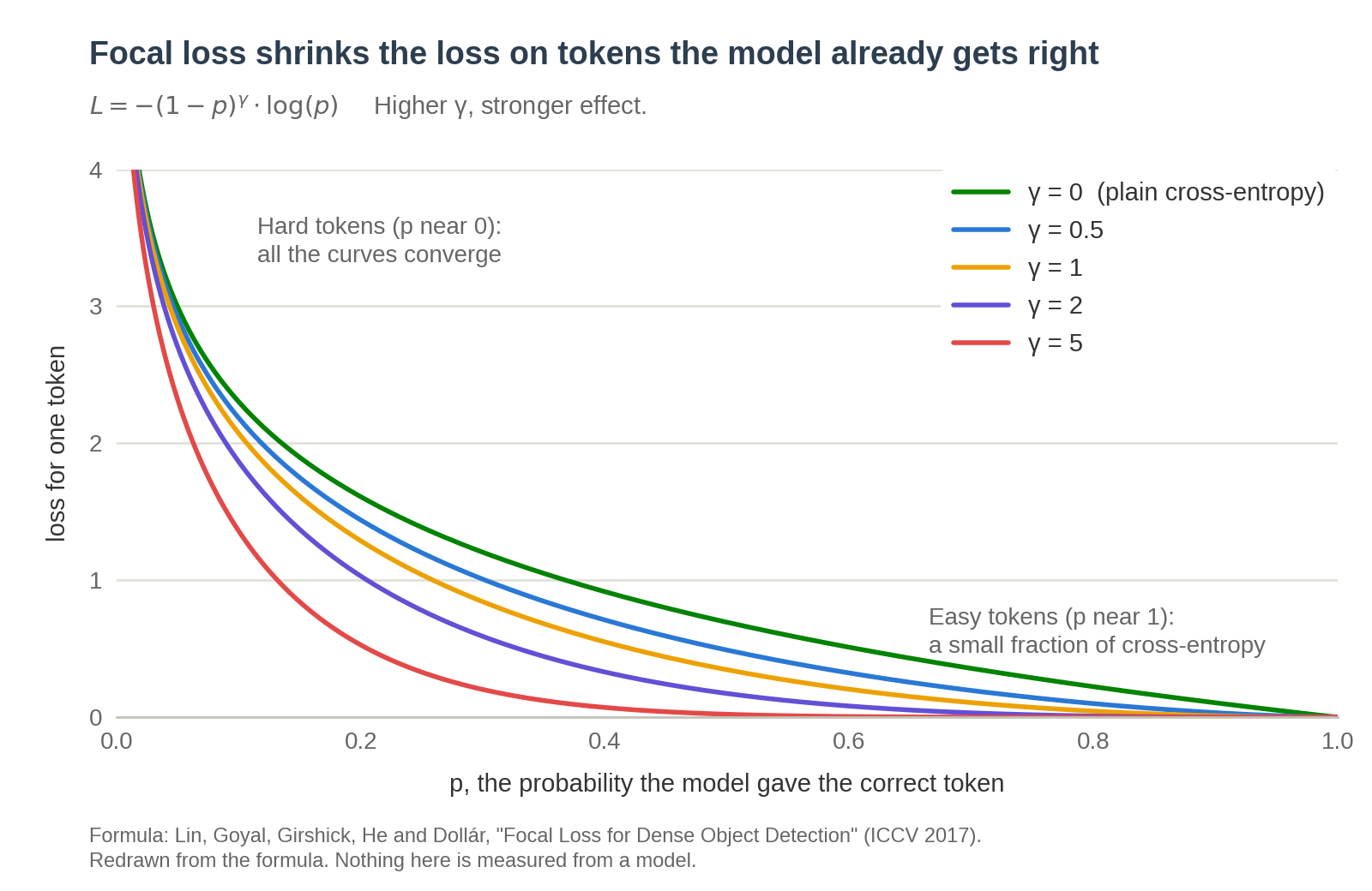
This chart is the paper's formula, redrawn by me. It is the same kind of plot as Figure 1 of the paper, which shows the loss for several values of gamma between 0 and 5. Nothing in it is measured from a model.
Side by side: the gradient
The loss value is not what trains the model. The gradient is. Write z for the logits, p_j for the softmax probability of token j, and t for the correct token, so p = p_t.
| Cross-entropy | Focal loss | |
|---|---|---|
Gradient on logit j |
p_j - [j = t] |
c(p) · (p_j - [j = t]) |
with
c(p) = (1 - p)^γ - γ · (1 - p)^(γ - 1) · p · log(p)
[j = t] is 1 for the correct token and 0 for every other token. Neither gradient is my result. The cross-entropy one is in every textbook, and the focal one is the paper's: its Appendix B gives it for the binary case, and the expression above is the same thing written for a softmax. I did not work it out with pencil and paper. I take the closed form and check it against PyTorch's autograd, which computes the same gradient its own way. The two agree to float32 rounding, and the check is further down, in the section on the variant that skips the float32 logits.
This is the part I find most useful for intuition. For any one token, focal loss pushes the logits in exactly the same direction as cross-entropy. It only rescales that token's push by c(p). Since log(p) is never positive, c(p) is never negative, so no token is ever pushed the wrong way. Focal loss is cross-entropy with a per-token learning rate that the model's own confidence sets.
The scale c(p), computed from that formula, for a few values of gamma:
| p | γ = 0 | γ = 0.5 | γ = 1 | γ = 2 | γ = 3 | γ = 5 |
|---|---|---|---|---|---|---|
| 0.01 | 1.000 | 1.018 | 1.036 | 1.071 | 1.106 | 1.172 |
| 0.10 | 1.000 | 1.070 | 1.130 | 1.224 | 1.289 | 1.346 |
| 0.30 | 1.000 | 1.053 | 1.061 | 0.996 | 0.874 | 0.602 |
| 0.50 | 1.000 | 0.952 | 0.847 | 0.597 | 0.385 | 0.140 |
| 0.90 | 1.000 | 0.466 | 0.195 | 0.029 | 0.0038 | 0.00006 |
| 0.95 | 1.000 | 0.333 | 0.099 | 0.0074 | 0.0005 | 0.000002 |
| 0.99 | 1.000 | 0.150 | 0.020 | 0.0003 | 0.000004 | below 0.000001 |
Three things to read off this table:
- Hard tokens get slightly more than cross-entropy gives them. At γ = 2 the scale peaks at about 1.22 near p = 0.10 and stays above 1 until p is about 0.30.
- Easy tokens get close to nothing. At γ = 2 a token at p = 0.95 gets under 1% of its cross-entropy gradient. Near p = 1 the scale is approximately
(1 + γ) · (1 - p)^γ. - Gamma above 2 starts cutting into the middle. At γ = 5 a token the model is only 50% sure of gets 14% of its cross-entropy gradient.
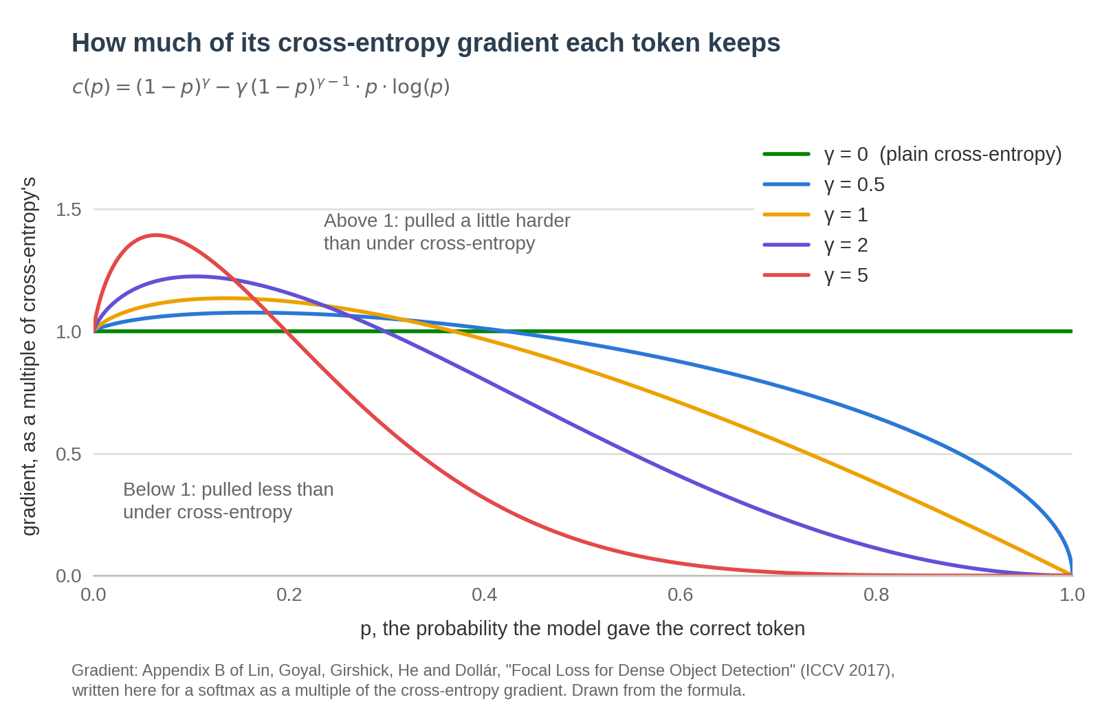
This chart is the table above as a picture. The gradient is the paper's, from its Appendix B, written here for a softmax and shown as a multiple of the cross-entropy gradient. I drew it from the formula, and nothing in it is measured from a model.
Side by side: the code
Plain cross-entropy in PyTorch is one call, F.cross_entropy(logits, targets, ignore_index=-100). Written out the long way, so that it lines up with the focal version, it is this. I wrote this one for the post, and it does what the built-in does:
import torch
import torch.nn.functional as F

def cross_entropy(logits, targets, ignore_index=-100):
    log_probs = F.log_softmax(logits.float(), dim=-1)

    valid_mask = (targets != ignore_index)
    safe_targets = targets.clone()
    safe_targets[~valid_mask] = 0

    # log(p) for the correct token at each position
    log_p = log_probs.gather(dim=-1, index=safe_targets.unsqueeze(-1)).squeeze(-1)

    loss = -log_p

    return loss[valid_mask].mean()
And this is the focal loss function from my project, with its comments shortened:
def focal_cross_entropy(logits, targets, gamma, ignore_index=-100, return_ce=False):
    """Focal loss: -(1-p)^gamma * log(p), mean over the valid positions.

    logits:  (N, vocab_size) unnormalized scores
    targets: (N,) correct token ids, ignore_index where the loss is masked
    gamma:   focusing parameter (0 = plain cross-entropy)
    return_ce: also return the plain cross-entropy, for the logs only
    """
    log_probs = F.log_softmax(logits.float(), dim=-1)

    valid_mask = (targets != ignore_index)
    safe_targets = targets.clone()
    safe_targets[~valid_mask] = 0

    # log(p) for the correct token at each position
    log_p = log_probs.gather(dim=-1, index=safe_targets.unsqueeze(-1)).squeeze(-1)

    # The modulator (1-p)^gamma. The clamp keeps gamma below 1 from
    # producing NaN gradients (see the next section).
    p = log_p.exp()
    focal_weight = (1.0 - p).clamp(min=1e-6) ** gamma

    loss = -focal_weight * log_p

    if valid_mask.any():
        focal = loss[valid_mask].mean()
    else:
        focal = loss.sum()
    if not return_ce:
        return focal

    # Plain cross-entropy from the log_p already gathered above.
    ce = (-log_p.detach()[valid_mask]).mean()
    return focal, ce
The whole difference between the two, as a diff:
-    loss = -log_p
+    p = log_p.exp()
+    focal_weight = (1.0 - p).clamp(min=1e-6) ** gamma
+    loss = -focal_weight * log_p
A few notes on the parts both versions share:
logits.float(): my models run in bfloat16, but the loss is computed in float32.1 - pfor a confident token is a tiny number and needs the precision.ignore_index: positions I do not train on (padding, and any position masked out of the loss) carry the target -100 and are left out of the mean.log_softmaxthenexp, notsoftmaxthenlog: the log-probability is the stable quantity, sopis derived from it and not the other way round.
In the model's forward pass, gamma arrives as an argument from the training loop. Simplified from my code:
if focal_gamma > 0:
    loss, ce_loss = focal_cross_entropy(flat_logits, flat_targets, focal_gamma, return_ce=True)
else:
    loss = F.cross_entropy(flat_logits, flat_targets, ignore_index=-100)
    ce_loss = loss.detach()
loss is what gets backpropagated. ce_loss goes to the logs. Gamma 0 takes the stock PyTorch path, so turning focal loss off is one setting and the result is exactly plain cross-entropy.
Addition 1: the clamp, or why gamma below 1 gave me NaN
On June 20, 2026 I woke up to a training run reporting NaN on its optimizer steps. My schedule used gamma values below 1 in parts of the run, and the model had become confident enough to expose a flaw in that.
The cause is in the gradient formula. The term γ · (1 - p)^(γ - 1) has a negative exponent when γ is below 1, so it grows without bound as p approaches 1. Mathematically that is harmless, because it is multiplied by log(p), which goes to zero faster, and the product goes to zero. Floating point does not take limits. The largest float32 below 1 is about 1 - 6e-8, so once the model is more certain than that about a token, p is exactly 1.0, 1 - p is exactly 0.0, autograd computes infinity for one factor and zero for the other, and infinity times zero is NaN. One such token poisons the whole batch. It only shows up once the model is good, because that is when tokens reach that level of certainty.
You can reproduce it in a few lines:
def grad_when_certain(gamma, clamp):
    logits = torch.tensor([[30.0, 0.0, 0.0]], requires_grad=True)  # certain of token 0
    log_p = F.log_softmax(logits, dim=-1)[0, 0]
    p = log_p.exp()                  # exactly 1.0 in float32
    base = 1.0 - p                   # exactly 0.0
    if clamp:
        base = base.clamp(min=1e-6)
    loss = -(base ** gamma) * log_p
    loss.backward()
    return logits.grad

print(grad_when_certain(0.5, clamp=False))   # tensor([[nan, nan, nan]])
print(grad_when_certain(0.5, clamp=True))    # tensor([[0.0000e+00, 9.3576e-17, 9.3576e-17]])
print(grad_when_certain(2.0, clamp=False))   # tensor([[0., 0., 0.]])
The fix is the .clamp(min=1e-6) on 1 - p. It keeps the base of the power away from zero, and inside the clamped range the clamp's own derivative is zero, which removes the infinity from the backward pass. A token that certain contributes next to nothing to the loss either way. With gamma at 1 or above the problem never arises, as the last line shows, which is why the paper's setting of 2 does not need this. A clamp like this is a routine numerical guard, not an invention. The point is that below 1 you need one.
Addition 2: train on the focal loss, read the cross-entropy
The first morning I had focal loss, I switched gamma from 0 to 2 in the middle of a run and within five steps the reported loss fell from 1.58 to 1.47. It took me a minute to see that the model had not suddenly improved. The ruler had changed.
The modulator is never above 1, so for the same model the focal loss is always at or below the cross-entropy, and the gap widens as the model gets more confident. That makes a focal loss number useless for comparison: against other people's models, against my own runs at a different gamma, even against the same run an hour earlier if gamma changed in between.
So my training loop keeps two numbers:
- the focal loss, which is backpropagated and which my schedule reads
- the plain cross-entropy, which is what gets printed, logged and charted
Since May 21, 2026 every loss I look at is true cross-entropy. At first that cost a second F.cross_entropy call on the same logits, purely for the log line. That is not cheap. A micro-batch of mine is 65,536 token positions against a 28,000-token vocabulary, and one float32 copy of those logits is 65,536 × 28,000 × 4 bytes = 7.3 GB. The second call made a second float32 cast and a second log-softmax, about 15 GB of short-lived GPU memory per micro-batch, to produce a number the focal pass already had in hand.
That is what return_ce=True is for. The focal pass has already gathered log(p) for every target, and plain cross-entropy is just the mean of -log(p). One line, the same value F.cross_entropy gives, no second pass.
Addition 3: gamma is scheduled, not fixed
Within an hour of the first commit I had moved gamma out of a constant and into my training schedule, and the reasoning has not changed: let the model learn the easy material first, then turn up the focus.
As I said at the top, changing gamma during training is not a new idea. This is just how I do it. I am not publishing my schedules, but the shape is simple:
- Start near zero. Through warm-up the loss is close to plain cross-entropy. A model that knows nothing has no easy tokens, and when the first ones appear (punctuation, the commonest words) I want them learned properly before they are downweighted.
- Raise gamma in steps as the loss falls. The schedule is driven by the training loss. Each time the loss crosses a threshold, gamma goes up a notch.
- Hold at 2.0 for the long middle. Most of the run is at the paper's value.
- Ease it back down at the end. In the final cool-down, as the learning rate comes down, gamma comes down with it, to below 1. This lets the easy tokens back in for the last stretch. It is also why I needed the clamp.
My first schedules pushed gamma up too hard and too early, and I backed that off within the first week.
A variant that skips the float32 logits
Because the gradient has the closed form above, the loss does not have to go through autograd at all. This function, a simplified version of what my trainer does that I wrote for this post, returns the gradient of the summed focal loss with respect to the logits directly:
def focal_grad_wrt_logits(logits, targets, gamma, clamp=1e-6):
    """dLoss/dlogits for the sum of the per-token focal losses (no masking, for clarity)."""
    log_probs = F.log_softmax(logits.float(), dim=-1)
    log_p = log_probs.gather(-1, targets.unsqueeze(-1)).squeeze(-1)
    p = log_p.exp()

    u = 1.0 - p
    uc = u.clamp(min=clamp)
    w = uc ** gamma                                    # the modulator
    dpow = torch.where(u >= clamp, gamma * uc ** (gamma - 1.0), torch.zeros_like(u))
    c = w - dpow * p * log_p                           # the per-token scale c(p)

    grad = log_probs.exp()                             # softmax
    grad[torch.arange(len(targets)), targets] -= 1.0   # minus 1 at the correct token
    return grad * c.unsqueeze(-1)
And here is the check against autograd, at gamma 2:
torch.manual_seed(0)
logits = (torch.randn(64, 50) * 4).requires_grad_(True)
targets = torch.randint(0, 50, (64,))

loss = focal_cross_entropy(logits, targets, gamma=2.0) * 64   # mean over 64 tokens, times 64 = the sum
loss.backward()                                                # autograd's gradient

mine = focal_grad_wrt_logits(logits.detach(), targets, gamma=2.0)
print((logits.grad - mine).abs().max())                        # tensor(1.1921e-07)
Across all 3,200 gradient entries, the largest difference between autograd and the closed form is one float32 rounding step.
My trainer has a version of this that works through the positions a chunk at a time, between the output layer's matrix multiplications, so the full float32 log-probabilities for every position never sit in memory at once. It gives the same loss and the same gradient to floating-point noise. It is a fallback: when the model is compiled with torch.compile, which is my normal setting and the faster of the two, the plain function above is the one that runs.
What I have measured
I have one controlled comparison, and I want to be exact about what it shows.
On a small pilot run of about a billion training tokens, I reran the back 40% of the run with gamma forced to 0, on the same code, data, batch sizes and learning rates. Both versions were then scored on the same five benchmarks. The difference, focal loss minus gamma 0, in points of accuracy:
| Benchmark | Focal loss minus gamma 0 | Standard error of that difference |
|---|---|---|
| HellaSwag | +0.11 | 0.15 |
| ARC-Easy | +0.25 | 0.37 |
| ARC-Challenge | -0.43 | 0.47 |
| PIQA | +0.33 | 0.43 |
| ArithMark-3 | -0.60 | 0.87 |
The standard error is the paired one. Both versions answer the same questions, so it counts only the questions where one was right and the other was wrong.
The focal run came out ahead on three of the five, and by 0.04 of a point on the Open SLM Index, the combined score that Boris-2's scoring procedure computes from them. Gamma 0 came out ahead on the other two. Every one of those differences is smaller than its own standard error, so the honest reading at this scale is a tie.
One more detail from that comparison is worth knowing. While the focal run sat at high gamma, its logged cross-entropy was slightly worse than the plain run's, by about 0.02, which is what you would expect from a loss that deliberately stops polishing easy tokens. The focal run's cool-down, where gamma eases back down, closed that gap to zero. So the cost of high gamma was real, small, and closed by the cool-down.
That is one pair of runs, with no repeats, and it was a brief test at a small scale. The pilot also spent only a small part of its length at gamma 2.0, where a full-length run spends most of it. My own expectation is that focal loss matters more over a full run. That is a belief and not a measurement.
The result I am really waiting for is how wayneworkman2012/boris2-peacebell-instruct turns out at full length. It is trained with focal loss, the same as Peacebell, where the original Boris-2-Instruct was trained with standard cross-entropy. Going the other way, Joseph Jones is building a Peacebell variant of his own with standard cross-entropy. Joseph and I are each using the other's data and tokenizer, and each keeping his own architecture and training regime. Neither will be a clean test of the loss, because his pipeline and mine differ in far more than that. But they are full-length runs, and that is where I expect to learn something.
If you want to try it
- Keep gamma 0 as a real option. It is exactly cross-entropy, so your baseline is one setting away. Run it.
- Do not start a from-scratch run at high gamma. Start near 0 and raise it as the loss falls.
- Treat 2.0 as the top. It is the paper's value and the highest I have trained with. The gradient table shows why I would not go higher: past 2 you stop downweighting easy tokens and start downweighting the ones the model is still unsure of.
- Below 1, clamp. If any part of your run uses gamma under 1, you need the clamp or something like it. The NaN will not show up early. It shows up when the model gets good.
- Log plain cross-entropy next to the focal loss. Take it from the same pass. Never compare focal loss values across different gammas.
- Know which number your tooling reads. A schedule, an early-stopping rule or an alert that watches the training loss will see it move every time gamma changes, with no change in the model.
- Ease gamma back down at the end if you care about likelihood-style scores such as perplexity or multiple-choice benchmarks scored by log-probability. High gamma leaves a little cross-entropy on the table and a low-gamma finish gets it back.
- Mind your data. Focal loss sends the gradient to whatever the model cannot predict. That includes the hard, valuable tokens, and it also includes errors in the training data. The cleaner the data, the better this trade is.
Timeline in my project
- March 5, 2026: focal loss committed ("implement focal loss gamma"). The same morning gamma moved into the training schedule.
- May 21, 2026: logs and metrics switched to true cross-entropy.
- June 20, 2026: the clamp, after an overnight run went NaN.
- September 14, 2026: the logged cross-entropy taken from the focal pass itself, removing the second pass.
- November 15, 2026: the chunked closed-form-gradient variant, and the first controlled comparison against gamma 0.
References
- Tsung-Yi Lin, Priya Goyal, Ross Girshick, Kaiming He, Piotr Dollár. "Focal Loss for Dense Object Detection." 2017 IEEE International Conference on Computer Vision (ICCV), 2017. https://arxiv.org/abs/1708.02002 (DOI: https://doi.org/10.1109/ICCV.2017.324). This is where focal loss comes from, and what everything in this post is based on.
Further reading, not something my implementation draws on:
- Jishnu Mukhoti, Viveka Kulharia, Amartya Sanyal, Stuart Golodetz, Philip H.S. Torr, Puneet K. Dokania. "Calibrating Deep Neural Networks using Focal Loss." NeurIPS 2020. https://arxiv.org/abs/2002.09437. A study of what focal loss does to how well a model's confidence matches its accuracy.
- Arindam Ghosh, Thomas Schaaf, Matthew R. Gormley. "AdaFocal: Calibration-aware Adaptive Focal Loss." NeurIPS 2022. https://arxiv.org/abs/2211.11838. One published way of adjusting gamma during training.